What This Document Is
This is a collection of worked examples focused on the application of state transition matrices within the field of mechanical systems. Specifically, it delves into methods for calculating these matrices, a crucial component in analyzing and predicting the behavior of dynamic systems. The examples are presented using the Mathematica computational software environment. It explores techniques for determining system responses based on initial conditions and input forces.
Why This Document Matters
This resource is ideal for students enrolled in courses like Mechanical Systems, Control Systems, or Dynamics. It’s particularly beneficial when you’re grappling with the practical implementation of theoretical concepts related to linear system analysis. If you're finding it difficult to translate equations of motion into a form suitable for state-space representation and subsequent analysis, this will be a valuable aid. It’s best used alongside your course textbook and lecture notes to reinforce understanding and build problem-solving skills. Students preparing for exams or tackling assignments involving system response analysis will find this particularly helpful.
Common Limitations or Challenges
This document focuses on *examples* of state transition matrix calculations. It does not provide a comprehensive derivation of the underlying theory. It assumes a foundational understanding of linear algebra, differential equations, and Laplace transforms. While the examples illustrate different system types, it doesn’t cover every possible scenario or system configuration. The use of Mathematica is central to the presentation; familiarity with the software is needed to fully utilize the material.
What This Document Provides
* Illustrative examples of state transition matrix calculations for various mechanical systems.
* Demonstrations of multiple methods for determining state transition matrices, including power series and eigenvalue-eigenvector approaches.
* Applications to specific systems, such as DC motors and inverted pendulums.
* Step-by-step implementations within the Mathematica environment.
* Comparisons of different solution techniques to highlight their strengths and weaknesses.